THIS POST IS PART OF OUR ANTHROPOCENE BIOSPHERE PROJECT–A SERIES OF POSTS ON ERLE ELLIS’ ‘ECOLOGY IN AN ANTHROPOGENIC BIOSPHERE‘ (ECOLOGICAL MONOGRAPHS, 85/3 (2015))

Ellis (2015) discusses in detail the idea that to be able to understand long-term ecological patterns and processes it is now necessary to understand human sociocultural processes first. To visualize the direct influence ofhumans on the landscape, Ellis and Ramankutty (2008) developed a dataset of anthropogenic biomes, which they shorten to “anthromes.” Anthromes are human biomes in which the global ecological patterns are classified according to the effect of human interactions with the ecosystems. Ellis et al. (2010) describes the development of these anthromes based on six underlying 5 by 5 minute spatial resolution datasets: population density (persons/km2), % cropland, % irrigated, % rice, % pasture and % urban. The anthromes papers (Ellis 2015; Ellis et al. 2010; Ellis and Ramankutty 2008) show the global distribution of these anthromes; however, to fully understand these datasets it is useful to take a closer look in a familiar area.

Below, I have extracted the anthromes for the four years (1700, 1800, 1900 and 2000) over Oklahoma as an illustration. There are a few things to notice in these maps. First, there is an interesting classification of Oklahoma’s land as ‘Inhabited treeless and barren lands’, while the land in Texas is classified as ‘Wild treeless and barren lands’ in 1700. A similar border can be found between Oklahoma and Arkansas, where the Oklahoma woodlands are classified as “Remote woodlands” while the Arkansas woodlands are classified as “Wild woodlands”. However, in general the 1700 data appear as expected. The subsequent maps show a slow but steady increase in the populated areas with the largest jump, as expected, between 1900 and 2000. By the year 2000 there are no treeless and barren lands left and all such land has been converted to croplands and rangelands or urban land. Similarly, most of the forests in the eastern portion of the state have been converted except for a small area in the southeastern part of the state.

Figure 1: Anthromes for Oklahoma, 1700.	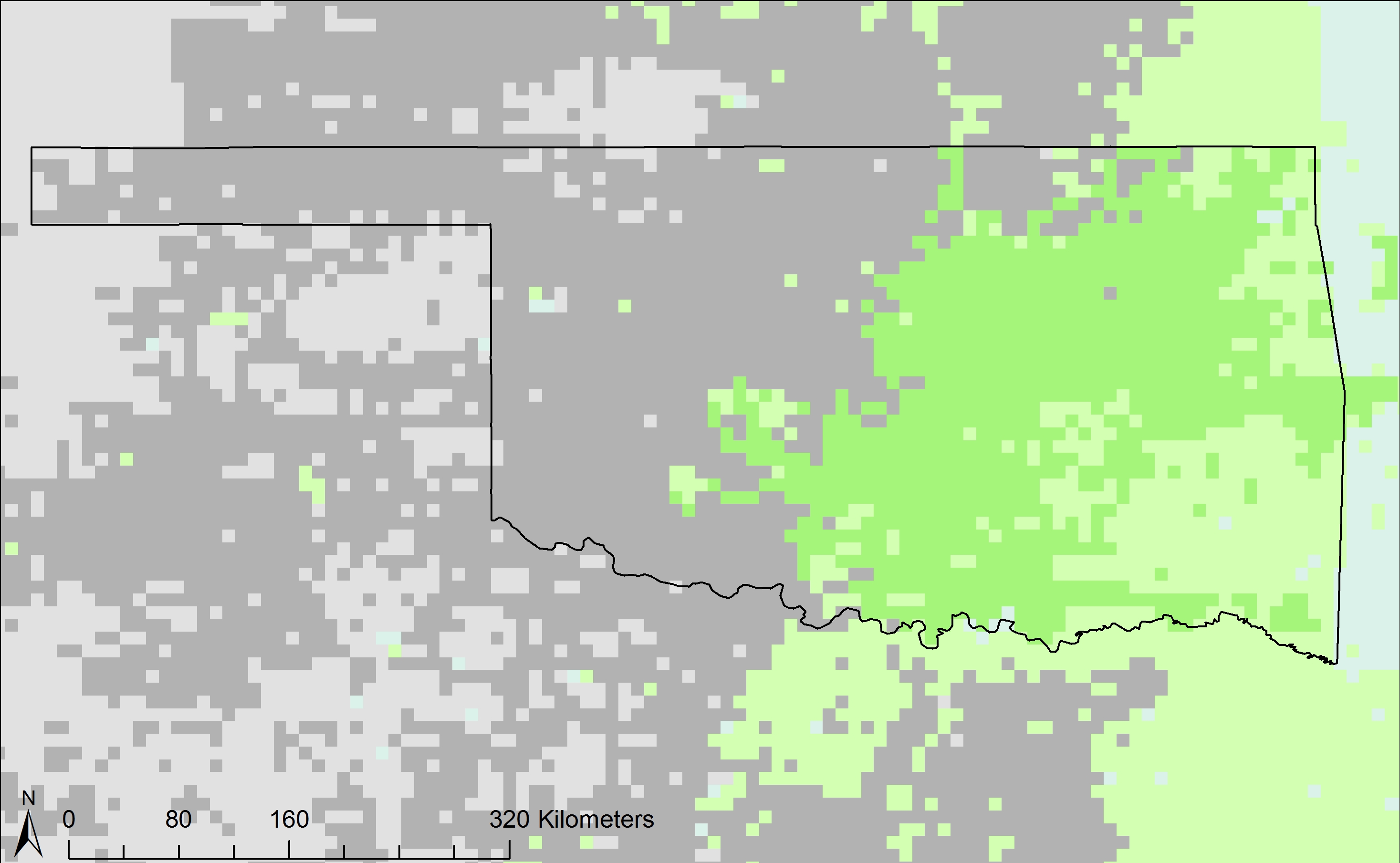Figure 2: Anthromes for Oklahoma, 1800.
Figure 3: Anthromes for Oklahoma, 1900.	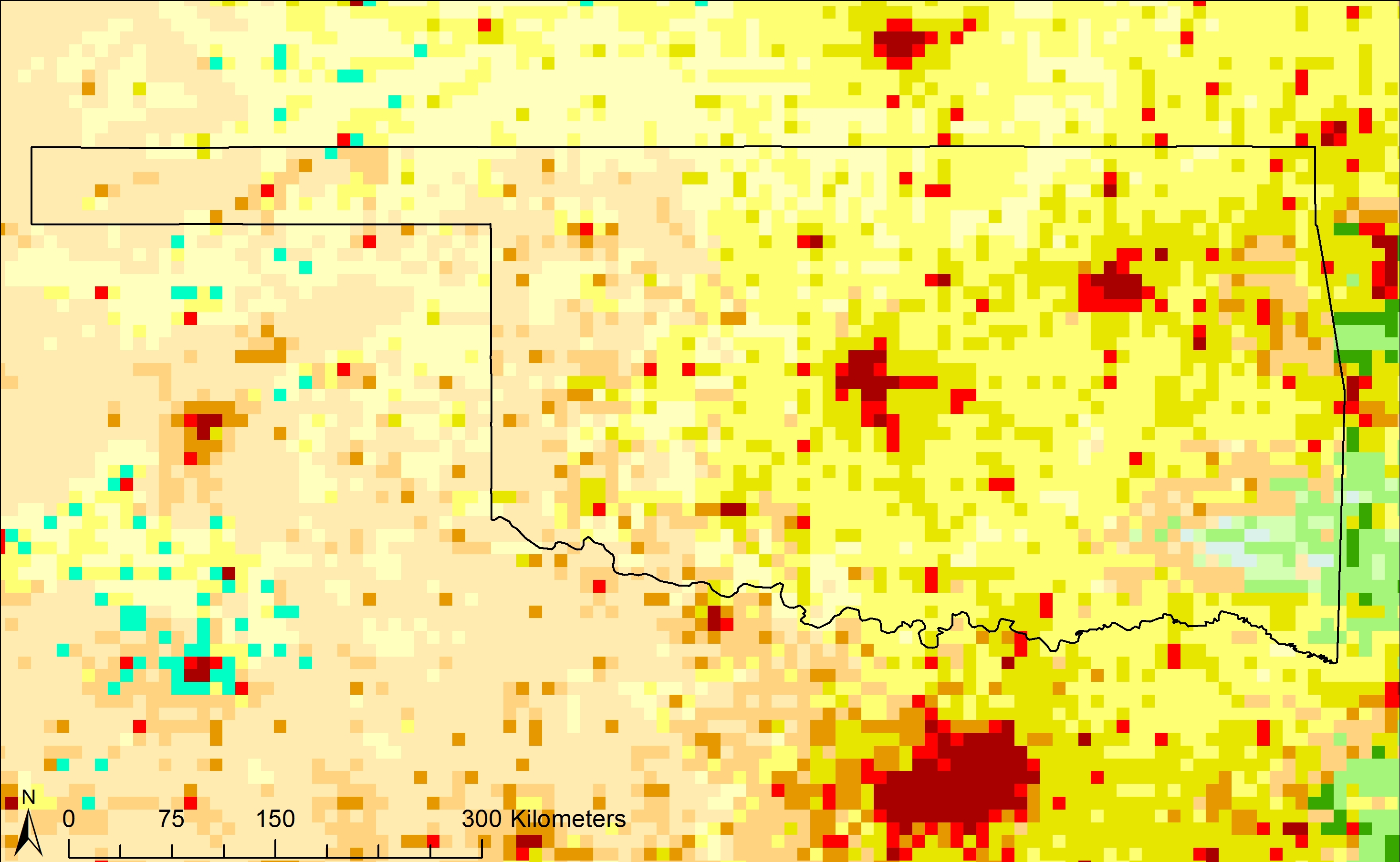Figure 4: Anthromes for Oklahoma, 2000.
Legend for figures 1-4.

If we graph the different classes over time, we can easily see the rapid decline in semi-natural lands between 1900 and 2000 in favor of croplands and rangelands.

Figure 5: Overview of changes in the anthromes for Oklahoma between 1700 and 2000.

Water Changes

One interesting feature to notice, especially for Oklahoma, is the omission of the increase in surface water on these maps. In a more detailed study for the Lake Thunderbird watershed we showed the change in stream channels for the Lake Thunderbird watershed in Central Oklahoma (Julian et al. 2015). This study shows much more detailed maps for Central Oklahoma and reveals a large increase in open water from less than 1% in the earliest maps (1874) to 6.9% of the watershed by 1975 which is mainly the result of the creation of Lake Stanley Draper in 1963 and Lake Thunderbird in 1965. Note that these lakes are invisible on the 2000 Anthromes map. Interesting especially because the lakes are man-made and one of the most important changes to the natural landscape over the past 100 years.

Spatial Resolution

The spatial resolution of the Anthromes data is 5 arc-minutes. This means that every grid cell measures 5 arc-minutes by 5 arc-minutes, which is approximately 9 by 9 km at the equator. In this day and age, spatial data are available at a range of different spatial resolutions. When evaluating changes on the land surface, it is often difficult to attribute the observed changes to either human or climatological factors. In a previous study we evaluated changes over a short time period (since 2000) at two spatial resolutions, 5.6km and 500m, in Russia and Kazakhstan (de Beurs et al. 2009). We found that the general pattern of observed changes is similar at the two spatial resolutions. The 5.6km spatial resolution is the current limit of regional and mesoscale meteorological models and we found that changes at this coarser scale are relevant to atmospheric boundary layer processes. The finer scale analysis however revealed trends that were more relevant to human decision-making and regional economics. As such we proposed that dual scale analysis might enable the partitioning of change attribution (de Beurs et al. 2009).

To provide a better understanding of the effect of different spatial resolutions, I show two maps with higher spatial resolution data for Oklahoma below. The first map provides the ambient population at a 1km2 spatial resolution from LandScan (Bright et al. 2011). This is a map for the year 2012 with every grid cell (1km by 1km) color coded according to its ambient population.

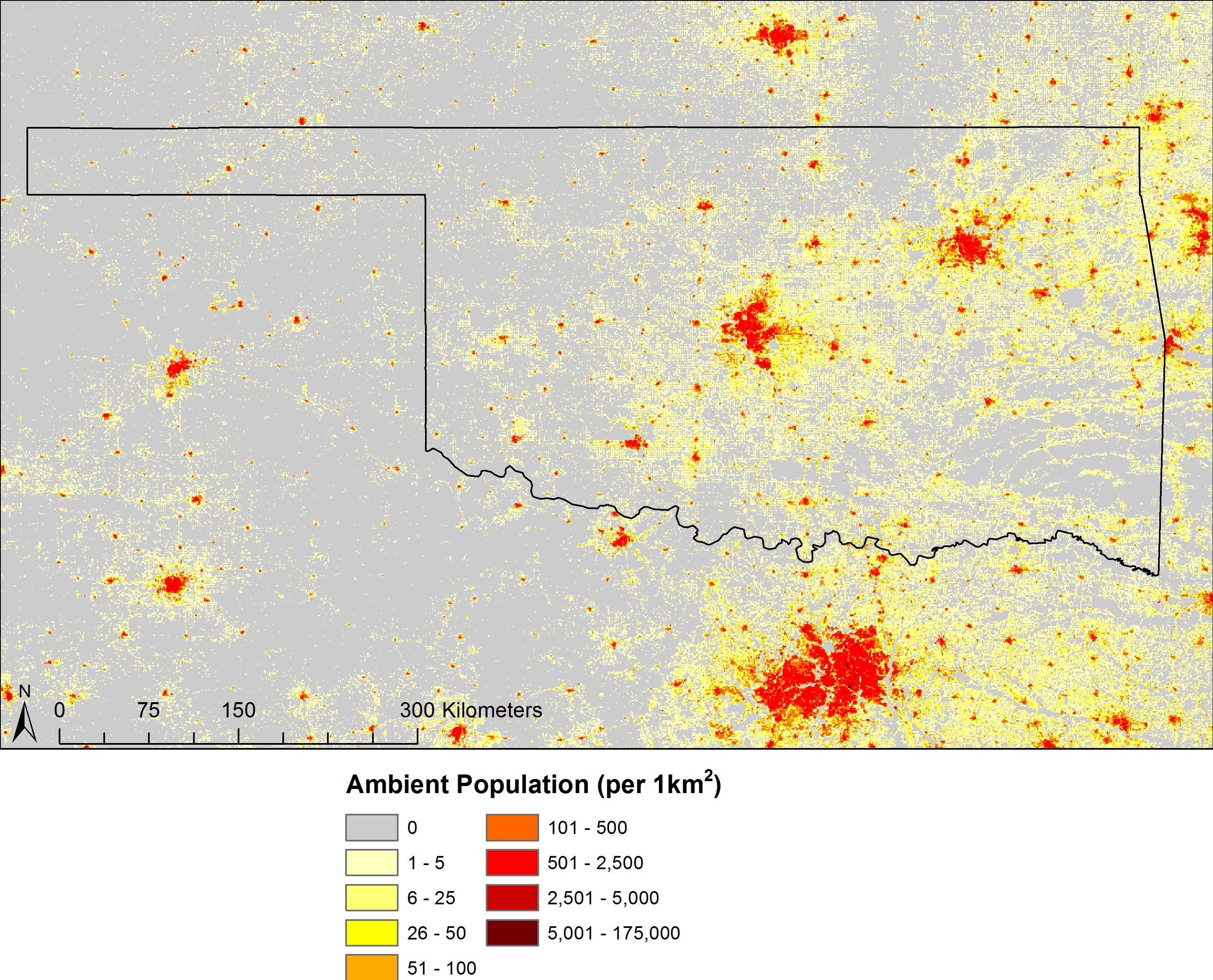
Figure 6: Ambient population from the LandScan data for Oklahoma, 2012. Spatial resolution: 1km.

The second map provides the impervious surface layer from the National Land Cover Dataset for Oklahoma (Homer et al. 2015). The spatial resolution of this data is 30m and every pixel is color coded according to the percentage of impervious surface. While human influence appears incredibly large and almost overpowering in the anthromes maps and even the Landscan data, the 30m resolution makes this influence look almost puny.

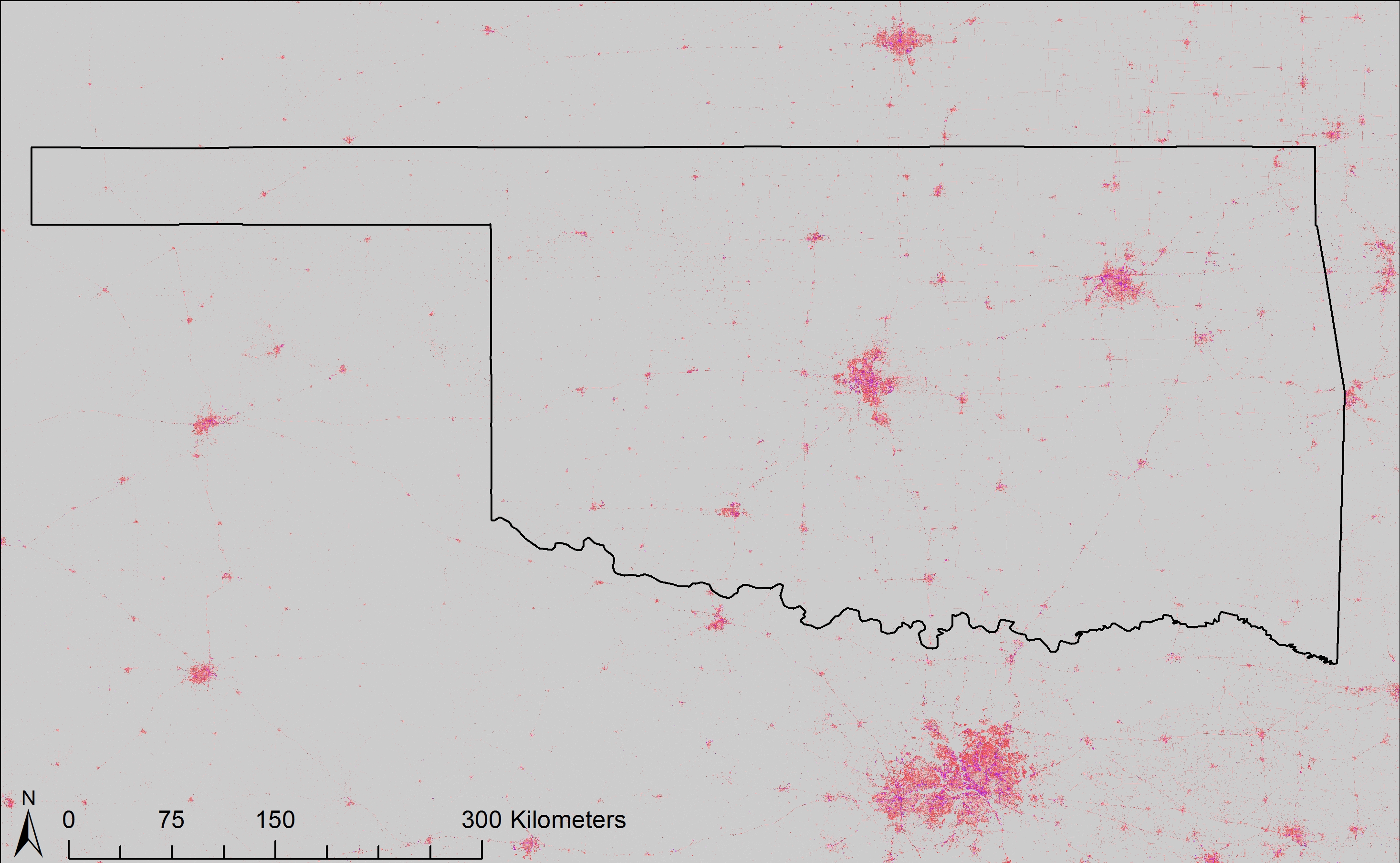
Figure 7: Percent impervious surface from the National Land Cover Dataset for Oklahoma, 2011. Spatial resolution: 30m.

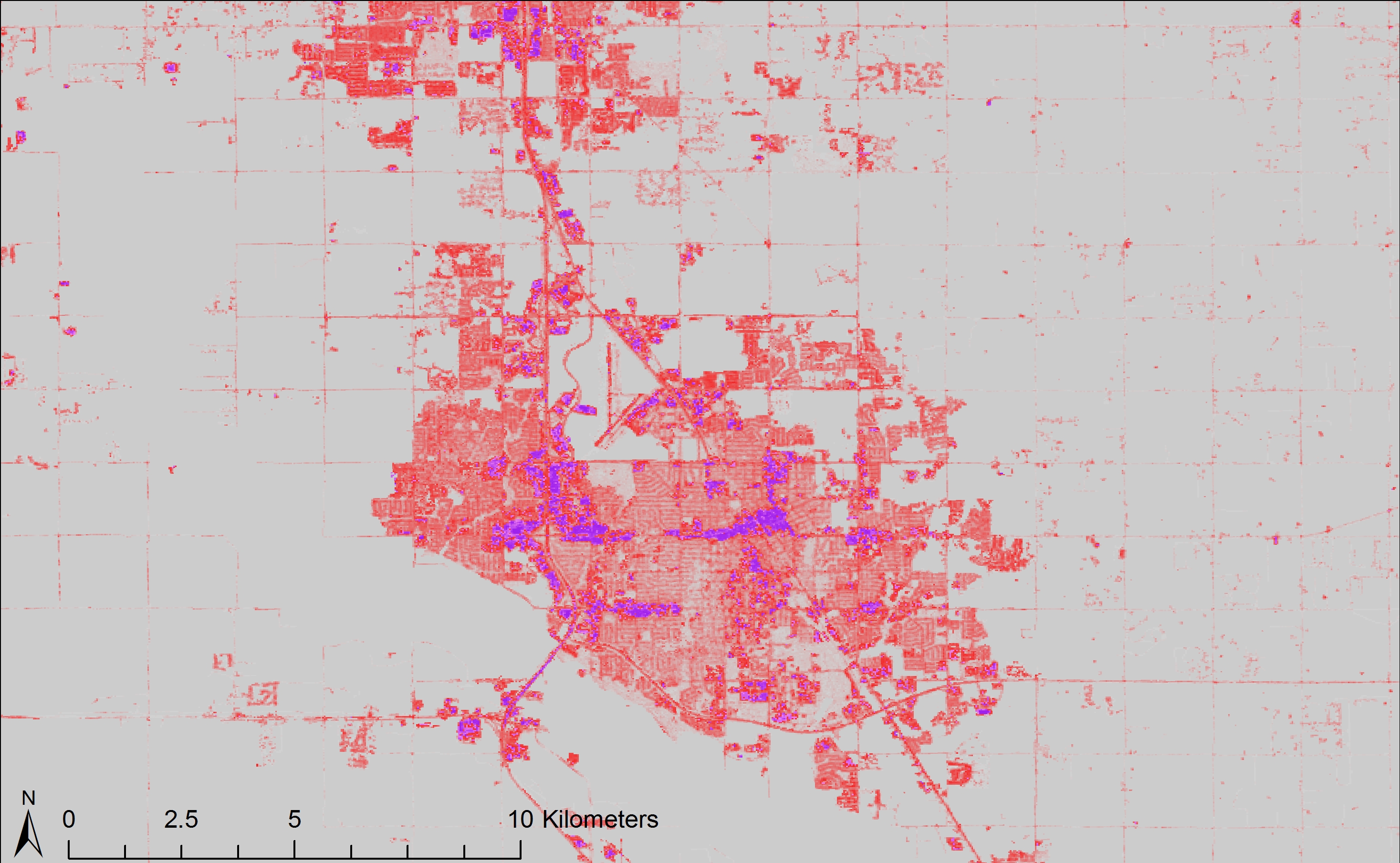
Figure 7 (detail): A zoom in to Norman (OK) for the 30m impervious data reveals the spatial detail of human influence.

References